Week 6

Data Wrangling and Visualization

Author

Prof. Jack Reilly

Published

Fall 2026

Problem Set 6 Solutions

This week’s solution is a small project rather than a single script: a master script that source()s a series of numbered scripts in order — load the data, manage it, draw the three figures in base R, in ggplot2, and in lattice, then explore two more variables — plus a Quarto write-up that pulls in the saved figures.

Download the whole project here — every script and the write-up, already laid out in the folder structure described below.

The scripts expect a particular folder structure

Every path in these scripts is relative to the project folder, so the layout has to be exactly this. Here is the folder as it looks on my machine:

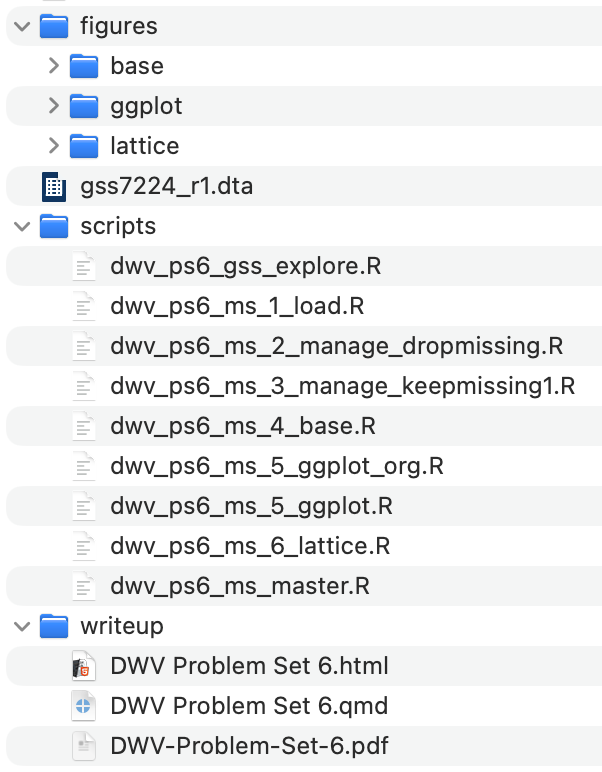
The project folder in Finder: a figures folder holding base, ggplot, and lattice subfolders; the GSS data file gss7224_r1.dta; a scripts folder holding the nine R scripts; and a writeup folder holding the html, qmd, and pdf of the write-up.

mondaksanders2026/           the project folder; the setwd() lines point here
    figures/base/            the scripts save their figures into these three folders
    figures/ggplot/
    figures/lattice/
    gss7224_r1.dta           the 1972-2024 cumulative GSS (not included; get it from gss.norc.org)
    scripts/                 all nine scripts, including dwv_ps6_ms_master.R, which sources the rest
    writeup/                 the Quarto write-up and its rendered .html and .pdf

The zip below unpacks into this layout, minus the data file (download it yourself) and the rendered .html (the master script’s last step produces it). Two lines to edit before running: the setwd() at the top of the master script, and the one in dwv_ps6_gss_explore.R, must point at wherever you put the folder. Note too that the master runs both ways of handling missing data (scripts 2 and 3); the second overwrites the first, so comment one out to choose.

The scripts

All nine live in the project’s scripts/ folder. Here they are in the order the master runs them.

Download dwv_ps6_ms_master.R

Preview: dwv_ps6_ms_master.R

dwv_ps6_ms_master.R

#Title: DWV Assign 6 - Mondak Sanders.R
#Author: Jack Reilly
#Purpose: Replicate Figures 1, 2, and 5 from Mondak & Sanders
#Requires: 1972-2024 Cumulative GSS Data ("gss7224_r1.dta"); expects a particular folder structure in home directory:
      # figures
        # base
        # ggplot
        # lattice
      # scripts
      # writeup
#Output: Figures as PDFs (ggplot only)

library(tidyverse)
library(haven)
library(quarto)

setwd("~/desktop/working/dwv/mondaksanders2026")

#Let's logically divide our tasks

# 1. Load data
# requires: working directory, libraries
# result: gss_subset
source("scripts/dwv_ps6_ms_1_load.R")

# We want to choose one style of missing data; run script 2 for removing all missing; script 3 for treating it like M&S

# 2. Manage data (missing=missing)
# requires: working directory, libraries, gss_subset
# result: gss_collapse (object for graphing) with missing=missing
source("scripts/dwv_ps6_ms_2_manage_dropmissing.R")

# 3. Manage data (missing=1)
# requires: working directory, libraries, gss_subset
# result: gss_collapse (object for graphing) with missing=1
source("scripts/dwv_ps6_ms_3_manage_keepmissing1.R")

# 3a. Regardless of which missing data style we're going to do, we want to get rid of those missing years
gss_collapse <- gss_collapse |>
  filter(!year %in% c(1978, 1983, 1986))

# 4. Draw data (base)
# requires: working directory, libraries, gss_collapse
# result: graphics in base R
pdf("figures/base/figures.pdf", width = 7, height = 5)
source("scripts/dwv_ps6_ms_4_base.R")
dev.off()

# 5. Draw data (ggplot2)
# requires: working directory, libraries, gss_collapse
# result: graphics in ggplot
source("scripts/dwv_ps6_ms_5_ggplot.R")

# 5a. Draw original data (ggplot2)
# requires: working directory, libraries, gss_collapse
# result: graphics in ggplot
source("scripts/dwv_ps6_ms_5_ggplot_org.R")

# 6. Draw data (lattice)
# requires: working directory, libraries, gss_collapse
# result: graphics in lattice
source("scripts/dwv_ps6_ms_6_lattice.R")

# 7. Make some other figures
source("scripts/dwv_ps6_gss_explore.R")

# 8. Render writeup
quarto::quarto_render("writeup/DWV Problem Set 6.qmd")

Download dwv_ps6_ms_1_load.R

Preview: dwv_ps6_ms_1_load.R

dwv_ps6_ms_1_load.R

#Title: dwv_ps6_ms_1_load.R
#Author: Jack Reilly
#Purpose: Load data
# requires: working directory, libraries
# result: gss_subset

gss<-read_dta("gss7224_r1.dta")

#Select the variables used by Mondak and Sanders, including the Year variable
#Mechanism: some of these show up in the codebook! But others don't.  
#Once you see the pattern, the rest are straightforward; missing ones can be found noted in GSS2024 Release Variables as dropped for the 2024 year
gss_sub <- gss |> select(year, spkath, colath, libath, spkrac, colrac, librac, spkcom, colcom, libcom, spkmil, colmil, libmil, spkhomo, colhomo, libhomo)

gss_sub <- filter(gss_sub, year >= 1976)

Download dwv_ps6_ms_2_manage_dropmissing.R

Preview: dwv_ps6_ms_2_manage_dropmissing.R

dwv_ps6_ms_2_manage_dropmissing.R

#Title: dwv_ps6_ms_2_dropmissing.R
#Author: Jack Reilly
#Purpose: Load data
# requires: working directory, libraries, gss_subset
# result: gss_collapse

#There is also an experiment the gss starts running with naming of these variables after 2021
#We'll ignore that and just look up to 2021

gss_sub <- filter(gss_sub, year >= 1976 & year <= 2021)


table(gss_sub$year)

table(gss_sub$colath)
unique(gss_sub$spkath)

gss_sub <- gss_sub |>
  mutate(
    ath1  = case_when(spkath == 1 ~ 0,
                      spkath == 2 ~ 1),
    ath2  = case_when(colath == 4 ~ 0,
                      colath == 5 ~ 1),
    ath3  = case_when(libath == 2 ~ 0,
                      libath == 1 ~ 1),
    
    rac1  = case_when(spkrac == 1 ~ 0,
                      spkrac == 2 ~ 1),
    rac2  = case_when(colrac == 4 ~ 0,
                      colrac == 5 ~ 1),
    rac3  = case_when(librac == 2 ~ 0,
                      librac == 1 ~ 1),
    
    com1  = case_when(spkcom == 1 ~ 0,
                      spkcom == 2 ~ 1),
    com2  = case_when(colcom == 5 ~ 0,   # note: colcom 4=1, 5=0
                      colcom == 4 ~ 1),
    com3  = case_when(libcom == 2 ~ 0,
                      libcom == 1 ~ 1),
    
    mil1  = case_when(spkmil == 1 ~ 0,
                      spkmil == 2 ~ 1),
    mil2  = case_when(colmil == 4 ~ 0,
                      colmil == 5 ~ 1),
    mil3  = case_when(libmil == 2 ~ 0,
                      libmil == 1 ~ 1),
    
    hom1 = case_when(spkhomo == 1 ~ 0,
                      spkhomo == 2 ~ 1),
    hom2 = case_when(colhomo == 4 ~ 0,
                      colhomo == 5 ~ 1),
    hom3 = case_when(libhomo == 2 ~ 0,
                      libhomo == 1 ~ 1)
  )

#Add all the variables together to make stouffer for fig1
gss_sub$stouffer <- gss_sub$ath1 + gss_sub$ath2 + gss_sub$ath3 + gss_sub$rac1 + gss_sub$rac2 + gss_sub$rac3 + gss_sub$com1 + gss_sub$com2 + gss_sub$com3 + gss_sub$mil1 + gss_sub$mil2 + gss_sub$mil3 + gss_sub$hom1 + gss_sub$hom2 + gss_sub$hom3
gss_sub$stouffer2 <- rowSums(gss_sub[, c("ath1", "ath2", "ath3", "rac1", "rac2", "rac3", "com1", "com2", "com3", "mil1", "mil2", "mil3", "hom1", "hom2", "hom3")], na.rm = TRUE)
gss_sub$stouffer3 <- rowSums(gss_sub[, c("ath1", "ath2", "ath3", "rac1", "rac2", "rac3", "com1", "com2", "com3", "mil1", "mil2", "mil3", "hom1", "hom2", "hom3")])

cor(gss_sub$stouffer, gss_sub$stouffer2, use = "pairwise.complete.obs")
cor(gss_sub$stouffer, gss_sub$stouffer3, use = "pairwise.complete.obs")
cor(gss_sub$stouffer2, gss_sub$stouffer3, use = "pairwise.complete.obs")

sum(!is.na(gss_sub$stouffer))
sum(!is.na(gss_sub$stouffer2))
sum(!is.na(gss_sub$stouffer3))

#What am I going to do here?
#Missing data management is important - here, I'm going to decide that I *just* want to have observations where I have complete data
#So I'm going to use the first or third commands

#Add rac and hom variables together for fig 2
gss_sub$rac = gss_sub$rac1 + gss_sub$rac2 + gss_sub$rac3
gss_sub$hom = gss_sub$hom1 + gss_sub$hom2 + gss_sub$hom3

#Generate intolerance variables - keep 0 as 0; keep missing as missing, else; turn into 1
gss_sub <- gss_sub |>
  mutate(
    intol = case_when(
      stouffer == 0 ~ 0,
      stouffer %in% 1:15 ~ 1  # everything else
    )
  )

#Look at our results
table(gss_sub$stouffer)
table(gss_sub$rac)
table(gss_sub$hom)
table(gss_sub$intol)

gss_collapse <- gss_sub |>
  group_by(year) |>
  summarize(
    stouffer = mean(stouffer, na.rm = T),
    rac = mean(rac, na.rm=T),
    hom = mean(hom, na.rm=T),
    intol = mean(intol, na.rm=T)
    )

table(gss_collapse$stouffer)
table(gss_collapse$rac)
table(gss_collapse$hom)
table(gss_collapse$intol)


plot(gss_collapse$year, gss_collapse$stouffer)
plot(gss_collapse$year, gss_collapse$rac)
plot(gss_collapse$year, gss_collapse$hom)
plot(gss_collapse$year, gss_collapse$intol)

Download dwv_ps6_ms_3_manage_keepmissing1.R

Preview: dwv_ps6_ms_3_manage_keepmissing1.R

dwv_ps6_ms_3_manage_keepmissing1.R

#Title: dwv_ps6_ms_3_keepmissing1.R
#Author: Jack Reilly
#Purpose: Load data
# requires: working directory, libraries, gss_subset
# result: gss_collapse

#So what haven't we done yet?
#Missing data - there are about 400 NA(d) in the spkath, for instance
table(na_tag(gss_sub$spkath))

gss_sub <- gss |> select(year, spkath, colath, libath, spkrac, colrac, librac, spkcom, colcom, libcom, spkmil, colmil, libmil, spkhomo, colhomo, libhomo)

#There is also an experiment the gss starts running with naming of these variables after 2021
#We'll ignore that and just look up to 2021

gss_sub <- filter(gss_sub, year >= 1976 & year <= 2021)

table(gss_sub$year)

gss_sub <- gss_sub |>
  mutate(
    ath1  = case_when(spkath == 1 ~ 0,
                      spkath == 2 ~ 1,
                      is_tagged_na(spkath) & na_tag(spkath) == "d" ~ 1),
    ath2  = case_when(colath == 4 ~ 0,
                      colath == 5 ~ 1,
                      is_tagged_na(colath) & na_tag(colath) == "d" ~ 1),
    ath3  = case_when(libath == 2 ~ 0,
                      libath == 1 ~ 1,
                      is_tagged_na(libath) & na_tag(libath) == "d" ~ 1),
    
    rac1  = case_when(spkrac == 1 ~ 0,
                      spkrac == 2 ~ 1,
                      is_tagged_na(spkrac) & na_tag(spkrac) == "d" ~ 1),
    rac2  = case_when(colrac == 4 ~ 0,
                      colrac == 5 ~ 1,
                      is_tagged_na(colrac) & na_tag(colrac) == "d" ~ 1),
    rac3  = case_when(librac == 2 ~ 0,
                      librac == 1 ~ 1,
                      is_tagged_na(librac) & na_tag(librac) == "d" ~ 1),
    
    com1  = case_when(spkcom == 1 ~ 0,
                      spkcom == 2 ~ 1,
                      is_tagged_na(spkcom) & na_tag(spkcom) == "d" ~ 1),
    com2  = case_when(colcom == 5 ~ 0,   # note: colcom 4=1, 5=0
                      colcom == 4 ~ 1,
                      is_tagged_na(colcom) & na_tag(colcom) == "d" ~ 1),
    com3  = case_when(libcom == 2 ~ 0,
                      libcom == 1 ~ 1,
                      is_tagged_na(libcom) & na_tag(libcom) == "d" ~ 1),
    
    mil1  = case_when(spkmil == 1 ~ 0,
                      spkmil == 2 ~ 1,
                      is_tagged_na(spkmil) & na_tag(spkmil) == "d" ~ 1),
    mil2  = case_when(colmil == 4 ~ 0,
                      colmil == 5 ~ 1,
                      is_tagged_na(colmil) & na_tag(colmil) == "d" ~ 1),
    mil3  = case_when(libmil == 2 ~ 0,
                      libmil == 1 ~ 1,
                      is_tagged_na(libmil) & na_tag(libmil) == "d" ~ 1),
    
    hom1 = case_when(spkhomo == 1 ~ 0,
                     spkhomo == 2 ~ 1,
                     is_tagged_na(spkhomo) & na_tag(spkhomo) == "d" ~ 1),
    hom2 = case_when(colhomo == 4 ~ 0,
                     colhomo == 5 ~ 1,
                     is_tagged_na(colhomo) & na_tag(colhomo) == "d" ~ 1),
    hom3 = case_when(libhomo == 2 ~ 0,
                     libhomo == 1 ~ 1,
                     is_tagged_na(libhomo) & na_tag(libhomo) == "d" ~ 1)
  )

#Generate our variables, like before
gss_sub$stouffer <- gss_sub$ath1 + gss_sub$ath2 + gss_sub$ath3 + gss_sub$rac1 + gss_sub$rac2 + gss_sub$rac3 + gss_sub$com1 + gss_sub$com2 + gss_sub$com3 + gss_sub$mil1 + gss_sub$mil2 + gss_sub$mil3 + gss_sub$hom1 + gss_sub$hom2 + gss_sub$hom3

gss_sub$rac = gss_sub$rac1 + gss_sub$rac2 + gss_sub$rac3
gss_sub$hom = gss_sub$hom1 + gss_sub$hom2 + gss_sub$hom3

#Generate intolerance variables - keep 0 as 0; keep missing as missing, else; turn into 1
gss_sub <- gss_sub |>
  mutate(
    intol = case_when(
      stouffer == 0 ~ 0,
      stouffer %in% 1:15 ~ 1  # everything else
    )
  )

#Look at our results
table(gss_sub$stouffer)
table(gss_sub$rac)
table(gss_sub$hom)
table(gss_sub$intol)

gss_collapse <- gss_sub |>
  group_by(year) |>
  summarize(
    stouffer = mean(stouffer, na.rm = TRUE),
    rac = mean(rac, na.rm=T),
    hom = mean(hom, na.rm=T),
    intol = mean(intol, na.rm=T)
  )

table(gss_collapse$stouffer)
table(gss_collapse$rac)
table(gss_collapse$hom)
table(gss_collapse$intol)


plot(gss_collapse$year, gss_collapse$stouffer)
plot(gss_collapse$year, gss_collapse$rac)
plot(gss_collapse$year, gss_collapse$hom)
plot(gss_collapse$year, gss_collapse$intol)

Download dwv_ps6_ms_4_base.R

Preview: dwv_ps6_ms_4_base.R

dwv_ps6_ms_4_base.R

#Title: dwv_ps6_ms_4_base.R
#Author: Jack Reilly
#Purpose: Load data
# requires: working directory, libraries, gss_collapse
# result: fig1, 2, 5 in base R (to viewer)

#Figure 1
#Let's do it properly nice, with layering in base R

plot(x=0, type='n',
     xlim=c(1976, 2021), xaxt = "n",
     ylim=c(0,15), yaxt = "n",
     xlab="Year", 
     ylab="Stouffer", 
     main="Figure 1. The 0-15 GSS Modified Stouffer Tolerance Battery, 1976-2021")

axis(1, at = c(1976, 2021)) #1 says "bottom axis"
axis(2, at = c(0, 15)) #2 says "left axis"

lines(gss_collapse$year, gss_collapse$stouffer, lwd=2)

#We gotta do it the real way this time
#Why? we don't know which version of the data we're getting - this will reflect whatever it is
v77<-gss_collapse$stouffer[gss_collapse$year == 1977]
v98<-gss_collapse$stouffer[gss_collapse$year == 1998]
v21<-gss_collapse$stouffer[gss_collapse$year == 2021]

#Round and paste it in
text(1985, 8, paste(round(v77, 2), "(1977)"))
text(1990, 3.5, paste(round(v98, 2), "(1998)"))
text(2014, 3.1, paste(round(v21, 2), "(2021)"))

#Let's get those arrows on

arrows(x0 = 1981.5, y0=7.8, x1=1977.5, y1=7,
       length = 0.1,  # length of arrowhead
       angle  = 30,   # angle of arrowhead
       code   = 2,    # 1 = head at x0,y0; 2 = head at x1,y1; 3 = both
       col    = "black", lwd = 1)

arrows(x0 = 1993.5, y0=3.7, x1=1997.5, y1=4.5,
       length = 0.1,  # length of arrowhead
       angle  = 30,   # angle of arrowhead
       code   = 2,    # 1 = head at x0,y0; 2 = head at x1,y1; 3 = both
       col    = "black", lwd = 1)

arrows(x0 = 2017, y0=3.2, x1=2020.5, y1=4.0,
       length = 0.1,  # length of arrowhead
       angle  = 30,   # angle of arrowhead
       code   = 2,    # 1 = head at x0,y0; 2 = head at x1,y1; 3 = both
       col    = "black", lwd = 1)

#Aha! 

#Figure 2

#Layer time
plot(x=0, type='n',
     xlim=c(1976, 2021), xaxt = "n",
     ylim=c(0,3), yaxt = "n",
     xlab=" ", 
     ylab=" ", 
     main="Figure 2. Intolerance Toward Racists and Homosexuals, 1976-2021")

axis(1, at = c(1976, 2021)) #1 says "bottom axis"
axis(2, at = c(0, 1, 2, 3)) #2 says "left axis"

lines(gss_collapse$year, gss_collapse$rac, lwd=2)
#lines(gss_collapse$year, gss_collapse$hom, lwd=2)
lines(gss_collapse$year, gss_collapse$hom, lwd=2, lty=2)

#Now all the text
#Nothing special to pull out here
text(1980, 1.5, "Racists")
text(1989, .7, "Homosexuals")


#Figure 5

#Layer time
plot(x=0, type='n',
     xlim=c(1976, 2021), xaxt = "n",
     ylim=c(0,1), yaxt = "n",
     xlab=" ", 
     ylab=" ", 
     main="Figure 5. A Dichotomous Measure of Tolerance and Intolerance, 1976-2021")

axis(1, at = c(1976, 2021)) #1 says "bottom axis"
axis(2, at = seq(0, 1, by = 0.1)) #2 says "left axis"

lines(gss_collapse$year, gss_collapse$intol, lwd=2)

Download dwv_ps6_ms_5_ggplot.R

Preview: dwv_ps6_ms_5_ggplot.R

dwv_ps6_ms_5_ggplot.R

#Title: dwv_ps6_ms_5_ggplot2.R
#Author: Jack Reilly
#Purpose: Load data
# requires: working directory, libraries, gss_collapse
# result: fig1, 2, 5 in ggplot2 (to viewer and wd)

##Let's do it in GGPlot

library(ggplot2)
library(grid)  # for unit() in arrow()

v77   <- gss_collapse$stouffer[gss_collapse$year == 1977]
v98   <- gss_collapse$stouffer[gss_collapse$year == 1998]
v21 <- gss_collapse$stouffer[gss_collapse$year == 2021]

fig1 <- ggplot(gss_collapse, aes(x = year, y = stouffer)) +
  geom_line(linewidth = 1) +
  scale_x_continuous(limits = c(1976, 2021), breaks = c(1976, 2021)) +
  scale_y_continuous(limits = c(0, 15), breaks = c(0, 15)) +
  labs(
    x = "Year",
    y = "Stouffer",
    title = "Figure 1. The 0-15 GSS Modified Stouffer Tolerance Battery, 1976-2021"
  ) +
  # text labels
  annotate("text", x = 1985, y = 8.0,  label = paste(round(v77, 2),   "(1977)")) +
  annotate("text", x = 1990, y = 3.5,  label = paste(round(v98, 2),   "(1998)")) +
  annotate("text", x = 2014, y = 3.1,  label = paste(round(v21, 2), "(2021)")) +
  # arrows (heads at xend,yend like code=2)
  annotate("segment",
           x = 1981.5, y = 7.8, xend = 1977.5, yend = 7.4,
           arrow = arrow(length = unit(0.1, "in"), angle = 30, ends = "last"),
           linewidth = 0.6, colour = "black") +
  annotate("segment",
           x = 1993.5, y = 3.7, xend = 1997.5, yend = 5.0,
           arrow = arrow(length = unit(0.1, "in"), angle = 30, ends = "last"),
           linewidth = 0.6, colour = "black") +
  annotate("segment",
           x = 2017.0, y = 3.5, xend = 2020.5, yend = 4.3,
           arrow = arrow(length = unit(0.1, "in"), angle = 30, ends = "last"),
           linewidth = 0.6, colour = "black") +
  theme_minimal(base_size = 12) +
  theme(panel.grid.minor = element_blank())

fig1
ggsave("figures/ggplot/figure1.pdf", fig1, width = 7.5, height = 7.55, dpi = 300)
ggsave("figures/ggplot/figure1.png", fig1, width = 7.5, height = 7.55, dpi = 300)

##Figure 2

fig2<-ggplot(gss_collapse, aes(x = year)) +
  # two lines
  geom_line(aes(y = rac), linewidth = 1) +
  geom_line(aes(y = hom), linewidth = 1, linetype = "dashed") +
  # scales with only endpoints / custom breaks
  scale_x_continuous(limits = c(1976, 2021), breaks = c(1976, 2021)) +
  scale_y_continuous(limits = c(0, 3), breaks = c(0, 1, 2, 3)) +
  # labels
  labs(
    x = NULL,
    y = NULL,
    title = "Figure 2. Intolerance Toward Racists and Homosexuals, 1976-2021"
  ) +
  # text annotations
  annotate("text", x = 1980, y = 1.5, label = "Racists") +
  annotate("text", x = 1989, y = 0.7, label = "Homosexuals") +
  theme_minimal(base_size = 12) +
  theme(panel.grid.minor = element_blank())

fig2
ggsave("figures/ggplot/figure2.pdf", fig2, width = 7.5, height = 7.55, dpi = 300)
ggsave("figures/ggplot/figure2.png", fig2, width = 7.5, height = 7.55, dpi = 300)


## Figure 5

fig5<-ggplot(gss_collapse, aes(x = year, y = intol)) +
  geom_line(linewidth = 1.2) +
  scale_x_continuous(limits = c(1976, 2021), breaks = c(1976, 2021)) +
  scale_y_continuous(limits = c(0, 1), breaks = seq(0, 1, by = 0.1)) +
  labs(
    x = NULL,
    y = NULL,
    title = "Figure 5. A Dichotomous Measure of Tolerance and Intolerance, 1976-2021"
  ) +
  theme_minimal(base_size = 12) +
  theme(panel.grid.minor = element_blank())

fig5
ggsave("figures/ggplot/figure5.pdf", fig5, width = 7.5, height = 7.55, dpi = 300)
ggsave("figures/ggplot/figure5.png", fig5, width = 7.5, height = 7.55, dpi = 300)

Download dwv_ps6_ms_5_ggplot_org.R

Preview: dwv_ps6_ms_5_ggplot_org.R

dwv_ps6_ms_5_ggplot_org.R

#Title: dwv_ps6_ms_5_ggplot2.R
#Author: Jack Reilly
#Purpose: Load data
# requires: working directory, libraries, gss_collapse
# result: fig1, 2, 5 in ggplot2 (to viewer and wd)

#Save the original collapse to restore at end of script
gss_collapse_save<-gss_collapse

#Get rid of later years for the "original" replication
gss_collapse <- gss_collapse |>
  filter(year <= 1998)

##Let's do it in GGPlot

library(ggplot2)
library(grid)  # for unit() in arrow()

v77   <- gss_collapse$stouffer[gss_collapse$year == 1977]
v98   <- gss_collapse$stouffer[gss_collapse$year == 1998]

fig1 <- ggplot(gss_collapse, aes(x = year, y = stouffer)) +
  geom_line(linewidth = 1) +
  scale_x_continuous(limits = c(1976, 1998), breaks = c(1976, 1998)) +
  scale_y_continuous(limits = c(0, 15), breaks = c(0, 15)) +
  labs(
    x = "Year",
    y = "Stouffer",
    title = "Figure 1. The 0-15 GSS Modified Stouffer Tolerance Battery, 1976-1998"
  ) +
  # text labels
  annotate("text", x = 1985, y = 8.0,  label = paste(round(v77, 2),   "(1977)")) +
  annotate("text", x = 1990, y = 3.5,  label = paste(round(v98, 2),   "(1998)")) +
    # arrows (heads at xend,yend like code=2)
  annotate("segment",
           x = 1981.5, y = 7.8, xend = 1977.5, yend = 7.4,
           arrow = arrow(length = unit(0.1, "in"), angle = 30, ends = "last"),
           linewidth = 0.6, colour = "black") +
  annotate("segment",
           x = 1993.5, y = 3.7, xend = 1997.5, yend = 5.0,
           arrow = arrow(length = unit(0.1, "in"), angle = 30, ends = "last"),
           linewidth = 0.6, colour = "black") +
  theme_minimal(base_size = 12) +
  theme(panel.grid.minor = element_blank())

fig1
ggsave("figures/ggplot/figure1_org.pdf", fig1, width = 7.5, height = 7.55, dpi = 300)
ggsave("figures/ggplot/figure1_org.png", fig1, width = 7.5, height = 7.55, dpi = 300)

##Figure 2

fig2<-ggplot(gss_collapse, aes(x = year)) +
  # two lines
  geom_line(aes(y = rac), linewidth = 1) +
  geom_line(aes(y = hom), linewidth = 1, linetype = "dashed") +
  # scales with only endpoints / custom breaks
  scale_x_continuous(limits = c(1976, 1998), breaks = c(1976, 1998)) +
  scale_y_continuous(limits = c(0, 3), breaks = c(0, 1, 2, 3)) +
  # labels
  labs(
    x = NULL,
    y = NULL,
    title = "Figure 2. Intolerance Toward Racists and Homosexuals, 1976-1998"
  ) +
  # text annotations
  annotate("text", x = 1980, y = 1.5, label = "Racists") +
  annotate("text", x = 1989, y = 0.7, label = "Homosexuals") +
  theme_minimal(base_size = 12) +
  theme(panel.grid.minor = element_blank())

fig2
ggsave("figures/ggplot/figure2_org.pdf", fig2, width = 7.5, height = 7.55, dpi = 300)
ggsave("figures/ggplot/figure2_org.png", fig2, width = 7.5, height = 7.55, dpi = 300)


## Figure 5

fig5<-ggplot(gss_collapse, aes(x = year, y = intol)) +
  geom_line(linewidth = 1.2) +
  scale_x_continuous(limits = c(1976, 1998), breaks = c(1976, 1998)) +
  scale_y_continuous(limits = c(0, 1), breaks = seq(0, 1, by = 0.1)) +
  labs(
    x = NULL,
    y = NULL,
    title = "Figure 5. A Dichotomous Measure of Tolerance and Intolerance, 1976-1998"
  ) +
  theme_minimal(base_size = 12) +
  theme(panel.grid.minor = element_blank())

fig5
ggsave("figures/ggplot/figure5_org.pdf", fig5, width = 7.5, height = 7.55, dpi = 300)
ggsave("figures/ggplot/figure5_org.png", fig5, width = 7.5, height = 7.55, dpi = 300)

gss_collapse<-gss_collapse_save

Download dwv_ps6_ms_6_lattice.R

Preview: dwv_ps6_ms_6_lattice.R

dwv_ps6_ms_6_lattice.R

#Title: dwv_ps6_ms_6_lattice.R
#Author: Jack Reilly
#Purpose: Load data
# requires: working directory, libraries, gss_collapse
# result: fig1, 2, 5 in lattice (to viewer to wd)

library(lattice)
library(grid)

v77   <- gss_collapse$stouffer[gss_collapse$year == 1977]
v98   <- gss_collapse$stouffer[gss_collapse$year == 1998]
v21 <- gss_collapse$stouffer[gss_collapse$year == 2021]

fig<-xyplot(
  stouffer ~ year,
  data = gss_collapse,
  type = "l",
  lwd = 2,
  xlab = "Year",
  ylab = "Stouffer",
  main = "Figure 1. The 0-15 GSS Modified Stouffer Tolerance Battery, 1976-2021",
  scales = list(
    x = list(limits = c(1976, 2021), at = c(1976, 2021)),
    y = list(limits = c(0, 15),      at = c(0, 15))
  ),
  panel = function(x, y, ...) {
    # line
    panel.xyplot(x, y, ...)
    
    # text labels
    panel.text(1985, 8, paste(round(v77, 2), "(1977)"))
    panel.text(1990, 3.5, paste(round(v98, 2), "(1998)"))
    panel.text(2014, 3.1, paste(round(v21, 2), "(2021)"))
    
    # arrows (arrowhead at end, like base code=2)
    panel.arrows(
      x0 = 1981.5, y0 = 7.8, x1 = 1977.5, y1 = 7.4,
      length = unit(0.1, "in"), angle = 30, ends = "last",
      col = "black", lwd = 1
    )
    panel.arrows(
      x0 = 1993.5, y0 = 3.7, x1 = 1997.5, y1 = 5.0,
      length = unit(0.1, "in"), angle = 30, ends = "last",
      col = "black", lwd = 1
    )
    panel.arrows(
      x0 = 2017.0, y0 = 3.5, x1 = 2020.5, y1 = 4.3,
      length = unit(0.1, "in"), angle = 30, ends = "last",
      col = "black", lwd = 1
    )
  }
)

fig

png("figures/lattice/fig1_lattice.png", width = 8, height = 5, units = "in", res = 300)
print(fig)
dev.off()

pdf("figures/lattice/fig1_lattice.pdf", width = 8, height = 5)
print(fig)
dev.off()

#Figure 2

fig<-xyplot(
  rac + hom ~ year,
  data = gss_collapse,
  type = "l",
  lwd = 1,
  lty = c(1, 2),  # solid for rac, dashed for hom
  scales = list(
    x = list(limits = c(1976, 2021), at = c(1976, 2021)),
    y = list(limits = c(0, 3), at = 0:3)
  ),
  xlab = "",
  ylab = "",
  main = "Figure 2. Intolerance Toward Racists and Homosexuals, 1976-2021",
  panel = function(x, y, ...) {
    panel.superpose(x, y, ...)  # draw the two series
    
    # add text labels directly
    panel.text(1980, 1.5, "Racists")
    panel.text(1989, 0.7, "Homosexuals")
  }
)

fig

png("figures/lattice/fig2_lattice.png", width = 8, height = 5, units = "in", res = 300)
print(fig)
dev.off()

pdf("figures/lattice/fig2_lattice.pdf", width = 8, height = 5)
print(fig)
dev.off()

#Figure 5 

fig<-xyplot(
  intol ~ year,
  data = gss_collapse,
  type = "l",
  col = "blue",
  lwd = 2,
  xlab = "Year",
  ylab = "Stouffer",
  main = "Figure 5. A Dichotomous Measure of Tolerance and Intolerance, 1976-2021",
  scales = list(
    x = list(limits = c(1976, 2021), at = c(1976, 2021)),
    y = list(limits = c(0, 1), at = seq(0, 1, by = 0.1))
  ),
  panel = function(x, y, ...) {
    panel.xyplot(x, y, ...)
  }
)

fig

png("figures/lattice/fig5_lattice.png", width = 8, height = 5, units = "in", res = 300)
print(fig)
dev.off()

pdf("figures/lattice/fig5_lattice.pdf", width = 8, height = 5)
print(fig)
dev.off()

Download dwv_ps6_gss_explore.R

Preview: dwv_ps6_gss_explore.R

dwv_ps6_gss_explore.R

#Title: DWV Assign 6 - Mondak Sanders.R
#Author: Jack Reilly
#Purpose: Explore two variables in the gss
#Requires: 1972-2024 Cumulative GSS Data ("gss7224_r1.dta"); expects a particular folder structure in home directory:
      # figures
        # base
        # ggplot
        # lattice
      # scripts
      # writeup
#Output: Figures as PDFs (ggplot only)

library(tidyverse)
library(lattice)

setwd("~/desktop/working/dwv/mondaksanders2026")

# Let's look at support for spending on space exploration

table(gss$natspac)
unique(gss$natspac)

histogram( ~ as.numeric(natspac), data=gss, xlab = "Support for Space Spending")

histogram(~ as.numeric(natspac), data = gss,
          breaks = seq(0.5, 3.5, by = 1),
          scales = list(x = list(at = 1:3,
                                 labels = c("Too little", "About right", "Too much"))),
          xlab = "Support for Space Spending")

gss_space <- gss |>
  mutate(natspac = as.numeric(natspac)) |>
  filter(natspac %in% 1:3) |>
  group_by(year) |>
  summarize(natspac = mean(natspac), n = n())

spaceplot<-ggplot(gss_space, aes(x = year, y = natspac)) +
  geom_line(linewidth = 1) +
  geom_point(size = 1.5) +
  scale_y_continuous(limits = c(1, 3), breaks = 1:3,
                     labels = c("Too little", "About right", "Too much")) +
  labs(x = NULL, y = NULL,
       title = "Averaged support for spending on space exploration") +
  theme_minimal() +
  theme(panel.grid.minor = element_blank())

sp2<-spaceplot+ theme(panel.grid.minor = element_blank(),
      panel.border = element_rect(colour = "black", fill = NA, linewidth = 0.5))

sp2

ggsave("figures/ggplot/spaceplot2.png", plot = sp2)

#Let's look at who believes the Earth goes around the Sun (and vice versa)

table(gss$earthsun)
unique(gss$earthsun)

histogram(~ as.numeric(earthsun), data = gss,
          breaks = c(0.5, 1.5, 2.5),
          scales = list(x = list(at = 1:2,
                                 labels = c("Earth goes around Sun", "Sun goes around Earth"))),
          xlab = "Does the Earth go around the Sun, or the Sun around the Earth?")

gss_earthsun <- gss |>
  mutate(earthsun = as.numeric(earthsun)) |>
  filter(earthsun %in% 1:2) |>
  group_by(year) |>
  summarize(correct = mean(earthsun == 1), n = n())

earthplot<-ggplot(gss_earthsun, aes(x = year, y = correct)) +
  geom_line(linewidth = 1) +
  geom_point(size = 1.5) +
  scale_y_continuous(limits = c(0, 1), labels = scales::percent) +
  labs(x = NULL, y = NULL,
       title = "Share answering that the Earth goes around the Sun") +
  theme_minimal() +
  theme(panel.grid.minor = element_blank())

ep2<-earthplot+ theme(panel.grid.minor = element_blank(),
      panel.border = element_rect(colour = "black", fill = NA, linewidth = 0.5))

ep2

ggsave("figures/ggplot/earthplot2.png", plot = ep2)

The write-up

Download the Quarto write-up and its rendered PDF. In the project it lives in writeup/ as DWV Problem Set 6.qmd, which is why its image paths start with ../figures/.

Preview: DWV Problem Set 6.qmd

DWV Problem Set 6.qmd

---
title: "Mondak & Sanders Replication"
author: Jack Reilly 
format: 
  html: 
    embed-resources: true
  pdf: default
---

What follows are three replications of Mondak & Sanders:

- Figure 1: The Modified Stouffer Tolerance Battery
- Figure 2: Intolerance Toward Racists and Homosexuals
- Figure 5: A Dichotomous Measure of Tolerance and Intolerance

## Figure 1

![Original](../figures/ggplot/figure1_org.png){fig-align="center" width="70%"}

![Expanded](../figures/ggplot/figure1.png){fig-align="center" width="70%"}

## Figure 2

![Original](../figures/ggplot/figure2_org.png){fig-align="center" width="70%"}

![Expanded](../figures/ggplot/figure2.png){fig-align="center" width="70%"}

## Figure 5

![Original](../figures/ggplot/figure5_org.png){fig-align="center" width="70%"}

![Expanded](../figures/ggplot/figure5.png){fig-align="center" width="70%"}

## Original Figures

![Support for Spending on Space Exploration](../figures/ggplot/spaceplot2.png){fig-align="center" width="70%"}

![% Who Correctly answer "Earth Goes Around the Sun"](../figures/ggplot/earthplot2.png){fig-align="center" width="70%"}


## Interpretive Questions

1. Everywhere.  I am become problems, destroyer of datasets.

2. Brief interpretations for each figure follow. 

  - Figure 1 - Intolerance continued declining, decreaseing from 7.24 in 1977 to 5.28 in 1998 to 4.43 in 2021.
  - Figure 2 - Intolerance toward racists maintained at steady levels; intolerance toward homosexuals continued falling.
  - Figure 3 - The dichotomous tolerance measure stayed pretty steady.

3. Kept slowly declining.

The single-file version

Download the single-file replication here — the same analysis as one long script, the way it was first worked out.

Prefer the project version

The project above is the better model: each step lives in its own small script, figures are saved to known folders, and the write-up is rebuilt from them, so any one step can be fixed or re-run without touching the rest. The single file does everything top to bottom — first rough drafts of each figure included — which reads well as a story but is hard to maintain; the figure labels, for instance, are typed in by hand rather than pulled from the data.

Preview: dwv_ps6_ms_singlefile.R

dwv_ps6_ms_singlefile.R

#Title: DWV Assign 6 - Mondak Sanders.R
#Author: Jack Reilly
#Purpose: Replicate Figures 1, 2, and 5 from Mondak & Sanders
#Requires: 1972-2024 Cumulative GSS Data ("gss7224_r1.dta")
#Output: Figures as PDFs (ggplot only)

library(tidyverse)
library(haven)

setwd("~/desktop/working/dwv/mondaksanders2026")

gss<-read_dta("gss7224_r1.dta")

#Select the variables used by Mondak and Sanders, including the Year variable
#Mechanism: some of these show up in the codebook! But others don't.  
#Once you see the pattern, the rest are straightforward; missing ones can be found noted in GSS2024 Release Variables as dropped for the 2024 year
gss_sub <- gss |> select(year, spkath, colath, libath, spkrac, colrac, librac, spkcom, colcom, libcom, spkmil, colmil, libmil, spkhomo, colhomo, libhomo)

gss_sub <- filter(gss_sub, year >= 1976)

table(gss_sub$year)

table(gss_sub$colath)
unique(gss_sub$spkath)

gss_sub <- gss_sub |>
  mutate(
    ath1  = case_when(spkath == 1 ~ 0,
                      spkath == 2 ~ 1),
    ath2  = case_when(colath == 4 ~ 0,
                      colath == 5 ~ 1),
    ath3  = case_when(libath == 2 ~ 0,
                      libath == 1 ~ 1),
    
    rac1  = case_when(spkrac == 1 ~ 0,
                      spkrac == 2 ~ 1),
    rac2  = case_when(colrac == 4 ~ 0,
                      colrac == 5 ~ 1),
    rac3  = case_when(librac == 2 ~ 0,
                      librac == 1 ~ 1),
    
    com1  = case_when(spkcom == 1 ~ 0,
                      spkcom == 2 ~ 1),
    com2  = case_when(colcom == 5 ~ 0,   # note: colcom 4=1, 5=0
                      colcom == 4 ~ 1),
    com3  = case_when(libcom == 2 ~ 0,
                      libcom == 1 ~ 1),
    
    mil1  = case_when(spkmil == 1 ~ 0,
                      spkmil == 2 ~ 1),
    mil2  = case_when(colmil == 4 ~ 0,
                      colmil == 5 ~ 1),
    mil3  = case_when(libmil == 2 ~ 0,
                      libmil == 1 ~ 1),
    
    hom1 = case_when(spkhomo == 1 ~ 0,
                      spkhomo == 2 ~ 1),
    hom2 = case_when(colhomo == 4 ~ 0,
                      colhomo == 5 ~ 1),
    hom3 = case_when(libhomo == 2 ~ 0,
                      libhomo == 1 ~ 1)
  )

#Add all the variables together to make stouffer for fig1
gss_sub$stouffer <- gss_sub$ath1 + gss_sub$ath2 + gss_sub$ath3 + gss_sub$rac1 + gss_sub$rac2 + gss_sub$rac3 + gss_sub$com1 + gss_sub$com2 + gss_sub$com3 + gss_sub$mil1 + gss_sub$mil2 + gss_sub$mil3 + gss_sub$hom1 + gss_sub$hom2 + gss_sub$hom3
gss_sub$stouffer2 <- rowSums(gss_sub[, c("ath1", "ath2", "ath3", "rac1", "rac2", "rac3", "com1", "com2", "com3", "mil1", "mil2", "mil3", "hom1", "hom2", "hom3")], na.rm = TRUE)
gss_sub$stouffer3 <- rowSums(gss_sub[, c("ath1", "ath2", "ath3", "rac1", "rac2", "rac3", "com1", "com2", "com3", "mil1", "mil2", "mil3", "hom1", "hom2", "hom3")])

cor(gss_sub$stouffer, gss_sub$stouffer2, use = "pairwise.complete.obs")
cor(gss_sub$stouffer, gss_sub$stouffer3, use = "pairwise.complete.obs")
cor(gss_sub$stouffer2, gss_sub$stouffer3, use = "pairwise.complete.obs")

sum(!is.na(gss_sub$stouffer))
sum(!is.na(gss_sub$stouffer2))
sum(!is.na(gss_sub$stouffer3))

#What am I going to do here?
#Missing data management is important - here, I'm going to decide that I *just* want to have observations where I have complete data
#So I'm going to use the first or third commands

#Add rac and hom variables together for fig 2
gss_sub$rac = gss_sub$rac1 + gss_sub$rac2 + gss_sub$rac3
gss_sub$hom = gss_sub$hom1 + gss_sub$hom2 + gss_sub$hom3

#Generate intolerance variables - keep 0 as 0; keep missing as missing, else; turn into 1
gss_sub <- gss_sub |>
  mutate(
    intol = case_when(
      stouffer == 0 ~ 0,
      stouffer %in% 1:15 ~ 1  # everything else
    )
  )

#Look at our results
table(gss_sub$stouffer)
table(gss_sub$rac)
table(gss_sub$hom)
table(gss_sub$intol)

gss_collapse <- gss_sub |>
  group_by(year) |>
  summarize(
    stouffer = mean(stouffer, na.rm = T),
    rac = mean(rac, na.rm=T),
    hom = mean(hom, na.rm=T),
    intol = mean(intol, na.rm=T)
    )

table(gss_collapse$stouffer)
table(gss_collapse$rac)
table(gss_collapse$hom)
table(gss_collapse$intol)


plot(gss_collapse$year, gss_collapse$stouffer)
plot(gss_collapse$year, gss_collapse$rac)
plot(gss_collapse$year, gss_collapse$hom)
plot(gss_collapse$year, gss_collapse$intol)

#OK! We've made it to our first shot at the graphs.  Now it's time to correct some issues:

#Figure 1
#Make it nicer looking

plot(gss_collapse$year, gss_collapse$stouffer, type = "o", col = "blue",
     xlab = "Year", ylab = "Stouffer",
     main = "Mondak & Sanders Replication")

#Huh. There are some missing years
gss_collapse <- gss_collapse |>
  filter(!year %in% c(1978, 1983, 1986))

#Let's do it a little bit nicer
plot(gss_collapse$year, gss_collapse$stouffer, type = "l", col = "blue",
     xlab = "Year", ylab = "Stouffer",
     xlim = c(1976, 2021), ylim = c(0, 15),
     main = "Figure 1. The 0-15 GSS Modified Stouffer Tolerance Battery, 1976-2021")

#Let's do it properly nicer, with layering in base R

plot(x=0, type='n',
     xlim=c(1976, 2021), xaxt = "n",
     ylim=c(0,15), yaxt = "n",
     xlab="Year", 
     ylab="Stouffer", 
     main="Figure 1. The 0-15 GSS Modified Stouffer Tolerance Battery, 1976-2021")

axis(1, at = c(1976, 2021)) #1 says "bottom axis"
axis(2, at = c(0, 15)) #2 says "left axis"

lines(gss_collapse$year, gss_collapse$stouffer, lwd=2)
#points(gss_collapse$year, gss_collapse$stouffer)

#Let's put those arrows on anyways!
#use to check positioning
#text(1985, 8, "I want it that way", col = "firebrick3")


#Actual
#text(1985, 8, "I want it that way", col = "firebrick3")
#text(1990, 3.5, "I want it that way", col = "firebrick3")
#text(2010, 2.5, "I want it that way", col = "firebrick3")

#This is kind of a clunky procedure anwyays. So I'm not going to worry about doing this in an internal, "pull the number from here" way
#I'm just going to look it up and put it in
print(gss_collapse, n=30)

#1977 is 6.84!
#1998 is 4.61!
#2021 is 4.41!

text(1985, 8, "6.84 (1977)")
text(1990, 3.5, "4.61 (1998)")
text(2014, 3.1, "4.41 (2021)")

#alt, if I *really* wanted to
v77<-gss_collapse$stouffer[gss_collapse$year == 1977]
v98<-gss_collapse$stouffer[gss_collapse$year == 1998]
v21<-gss_collapse$stouffer[gss_collapse$year == 2021]

#I can use the paste command to stick things together in a string
#text(1985, 8, paste(v77, "(1977)"))

#Oops.  Let's not have so many digits.  We'll round
text(1985, 8, paste(round(v77, 2), "(1977)"))
text(1990, 3.5, paste(round(v98, 2), "(1998)"))
text(2014, 3.1, paste(round(v21, 2), "(2021)"))

#Let's get those arrows on

#Practice
#arrows(x0 = 1985, y0=9, x1=1984, y1=10,
#       length = 0.1,  # length of arrowhead
#       angle  = 30,   # angle of arrowhead
#       code   = 2,    # 1 = head at x0,y0; 2 = head at x1,y1; 3 = both
#       col    = "red", lwd = 2)

arrows(x0 = 1981.5, y0=7.8, x1=1977.5, y1=7,
       length = 0.1,  # length of arrowhead
       angle  = 30,   # angle of arrowhead
       code   = 2,    # 1 = head at x0,y0; 2 = head at x1,y1; 3 = both
       col    = "black", lwd = 1)

arrows(x0 = 1993.5, y0=3.7, x1=1997.5, y1=4.5,
       length = 0.1,  # length of arrowhead
       angle  = 30,   # angle of arrowhead
       code   = 2,    # 1 = head at x0,y0; 2 = head at x1,y1; 3 = both
       col    = "black", lwd = 1)

arrows(x0 = 2017, y0=3.2, x1=2020.5, y1=4.0,
       length = 0.1,  # length of arrowhead
       angle  = 30,   # angle of arrowhead
       code   = 2,    # 1 = head at x0,y0; 2 = head at x1,y1; 3 = both
       col    = "black", lwd = 1)

#Haha! 

#Figure 2
plot(gss_collapse$year, gss_collapse$rac, type = "l", col = "blue",
     xlab = "Year", ylab = "Stouffer",
     xlim = c(1976, 2021), ylim = c(0, 3),
     main = "Figure 2. Intolerance Toward Racists and Homosexuals, 1976-2021")

plot(gss_collapse$year, gss_collapse$hom, type = "l", col = "blue",
     xlab = "Year", ylab = "Stouffer",
     xlim = c(1976, 2021), ylim = c(0, 3),
     main = "Figure 2. Intolerance Toward Racists and Homosexuals, 1976-2021")

#Layer time
plot(x=0, type='n',
     xlim=c(1976, 2021), xaxt = "n",
     ylim=c(0,3), yaxt = "n",
     xlab=" ", 
     ylab=" ", 
     main="Figure 2. Intolerance Toward Racists and Homosexuals, 1976-2021")

axis(1, at = c(1976, 2021)) #1 says "bottom axis"
axis(2, at = c(0, 1, 2, 3)) #2 says "left axis"

lines(gss_collapse$year, gss_collapse$rac, lwd=2)
#lines(gss_collapse$year, gss_collapse$hom, lwd=2)
lines(gss_collapse$year, gss_collapse$hom, lwd=2, lty=2)

#Oh no, now all the text

text(1980, 1.5, "Racists")
text(1989, .7, "Homosexuals")


#Figure 5
plot(gss_collapse$year, gss_collapse$intol, type = "l", col = "blue",
     xlab = "Year", ylab = "Stouffer",
     xlim = c(1976, 2021), ylim = c(0, 1),
     main = "Figure 5. A Dichotomous Measure of Tolerance and Intolerance, 1976-2021")

#Layer time
plot(x=0, type='n',
     xlim=c(1976, 2021), xaxt = "n",
     ylim=c(0,1), yaxt = "n",
     xlab=" ", 
     ylab=" ", 
     main="Figure 5. A Dichotomous Measure of Tolerance and Intolerance, 1976-2021")

axis(1, at = c(1976, 2021)) #1 says "bottom axis"
axis(2, at = seq(0, 1, by = 0.1)) #2 says "left axis"

lines(gss_collapse$year, gss_collapse$intol, lwd=2)


#So what haven't we done yet?
#Missing data - there are about 400 NA(d) in the spkath, for instance
table(na_tag(gss_sub$spkath))

gss_sub <- gss |> select(year, spkath, colath, libath, spkrac, colrac, librac, spkcom, colcom, libcom, spkmil, colmil, libmil, spkhomo, colhomo, libhomo)

#There is also an experiment the gss starts running with naming of these variables after 2021
#We'll ignore that for now and just look up to 2021

gss_sub <- filter(gss_sub, year >= 1976 & year <= 2021)

table(gss_sub$year)

gss_sub <- gss_sub |>
  mutate(
    ath1  = case_when(spkath == 1 ~ 0,
                      spkath == 2 ~ 1,
                      is_tagged_na(spkath) & na_tag(spkath) == "d" ~ 1),
    ath2  = case_when(colath == 4 ~ 0,
                      colath == 5 ~ 1,
                      is_tagged_na(colath) & na_tag(colath) == "d" ~ 1),
    ath3  = case_when(libath == 2 ~ 0,
                      libath == 1 ~ 1,
                      is_tagged_na(libath) & na_tag(libath) == "d" ~ 1),
    
    rac1  = case_when(spkrac == 1 ~ 0,
                      spkrac == 2 ~ 1,
                      is_tagged_na(spkrac) & na_tag(spkrac) == "d" ~ 1),
    rac2  = case_when(colrac == 4 ~ 0,
                      colrac == 5 ~ 1,
                      is_tagged_na(colrac) & na_tag(colrac) == "d" ~ 1),
    rac3  = case_when(librac == 2 ~ 0,
                      librac == 1 ~ 1,
                      is_tagged_na(librac) & na_tag(librac) == "d" ~ 1),
    
    com1  = case_when(spkcom == 1 ~ 0,
                      spkcom == 2 ~ 1,
                      is_tagged_na(spkcom) & na_tag(spkcom) == "d" ~ 1),
    com2  = case_when(colcom == 5 ~ 0,   # note: colcom 4=1, 5=0
                      colcom == 4 ~ 1,
                      is_tagged_na(colcom) & na_tag(colcom) == "d" ~ 1),
    com3  = case_when(libcom == 2 ~ 0,
                      libcom == 1 ~ 1,
                      is_tagged_na(libcom) & na_tag(libcom) == "d" ~ 1),
    
    mil1  = case_when(spkmil == 1 ~ 0,
                      spkmil == 2 ~ 1,
                      is_tagged_na(spkmil) & na_tag(spkmil) == "d" ~ 1),
    mil2  = case_when(colmil == 4 ~ 0,
                      colmil == 5 ~ 1,
                      is_tagged_na(colmil) & na_tag(colmil) == "d" ~ 1),
    mil3  = case_when(libmil == 2 ~ 0,
                      libmil == 1 ~ 1,
                      is_tagged_na(libmil) & na_tag(libmil) == "d" ~ 1),
    
    hom1 = case_when(spkhomo == 1 ~ 0,
                     spkhomo == 2 ~ 1,
                     is_tagged_na(spkhomo) & na_tag(spkhomo) == "d" ~ 1),
    hom2 = case_when(colhomo == 4 ~ 0,
                     colhomo == 5 ~ 1,
                     is_tagged_na(colhomo) & na_tag(colhomo) == "d" ~ 1),
    hom3 = case_when(libhomo == 2 ~ 0,
                     libhomo == 1 ~ 1,
                     is_tagged_na(libhomo) & na_tag(libhomo) == "d" ~ 1)
  )

#Generate our variables, like before
gss_sub$stouffer <- gss_sub$ath1 + gss_sub$ath2 + gss_sub$ath3 + gss_sub$rac1 + gss_sub$rac2 + gss_sub$rac3 + gss_sub$com1 + gss_sub$com2 + gss_sub$com3 + gss_sub$mil1 + gss_sub$mil2 + gss_sub$mil3 + gss_sub$hom1 + gss_sub$hom2 + gss_sub$hom3

gss_sub$rac = gss_sub$rac1 + gss_sub$rac2 + gss_sub$rac3
gss_sub$hom = gss_sub$hom1 + gss_sub$hom2 + gss_sub$hom3

#Generate intolerance variables - keep 0 as 0; keep missing as missing, else; turn into 1
gss_sub <- gss_sub |>
  mutate(
    intol = case_when(
      stouffer == 0 ~ 0,
      stouffer %in% 1:15 ~ 1  # everything else
    )
  )

#Look at our results
table(gss_sub$stouffer)
table(gss_sub$rac)
table(gss_sub$hom)
table(gss_sub$intol)

gss_collapse <- gss_sub |>
  group_by(year) |>
  summarize(
    stouffer = mean(stouffer, na.rm = TRUE),
    rac = mean(rac, na.rm=T),
    hom = mean(hom, na.rm=T),
    intol = mean(intol, na.rm=T)
  )

table(gss_collapse$stouffer)
table(gss_collapse$rac)
table(gss_collapse$hom)
table(gss_collapse$intol)


plot(gss_collapse$year, gss_collapse$stouffer)
plot(gss_collapse$year, gss_collapse$rac)
plot(gss_collapse$year, gss_collapse$hom)
plot(gss_collapse$year, gss_collapse$intol)

#OK! We've made it to our first shot at the graphs.  Now it's time to correct some issues:

#Figure 1
#Make it nicer looking

plot(gss_collapse$year, gss_collapse$stouffer, type = "o", col = "blue",
     xlab = "Year", ylab = "Stouffer",
     main = "Mondak & Sanders Replication")

#Huh. There are some missing years
gss_collapse <- gss_collapse |>
  filter(!year %in% c(1978, 1983, 1986))

#Let's do it a little bit nicer
plot(gss_collapse$year, gss_collapse$stouffer, type = "l", col = "blue",
     xlab = "Year", ylab = "Stouffer",
     xlim = c(1976, 2021), ylim = c(0, 15),
     main = "Figure 1. The 0-15 GSS Modified Stouffer Tolerance Battery, 1976-2021")

#Let's do it properly nicer, with layering in base R

plot(x=0, type='n',
     xlim=c(1976, 2021), xaxt = "n",
     ylim=c(0,15), yaxt = "n",
     xlab="Year", 
     ylab="Stouffer", 
     main="Figure 1. The 0-15 GSS Modified Stouffer Tolerance Battery, 1976-2021")

axis(1, at = c(1976, 2021)) #1 says "bottom axis"
axis(2, at = c(0, 15)) #2 says "left axis"

lines(gss_collapse$year, gss_collapse$stouffer, lwd=2)
#points(gss_collapse$year, gss_collapse$stouffer)

#Let's put those arrows on anyways!
#use to check positioning
#text(1985, 8, "I want it that way", col = "firebrick3")


#Actual
#text(1985, 8, "I want it that way", col = "firebrick3")
#text(1990, 3.5, "I want it that way", col = "firebrick3")
#text(2010, 2.5, "I want it that way", col = "firebrick3")

#This is kind of a clunky procedure anwyays. So I'm not going to worry about doing this in an internal, "pull the nubmer from here" way
#I'm just going to look it up and put it in

print(gss_collapse, n=30)

#1977 is 6.84!
#1998 is 4.61!
#2021 is 4.41!

text(1985, 8, "7.24 (1977)")
text(1990, 3.5, "5.28 (1998)")
text(2014, 3.1, "4.43 (2021)")

#Let's get those arrows on

#Practice
#arrows(x0 = 1985, y0=9, x1=1984, y1=10,
#       length = 0.1,  # length of arrowhead
#       angle  = 30,   # angle of arrowhead
#       code   = 2,    # 1 = head at x0,y0; 2 = head at x1,y1; 3 = both
#       col    = "red", lwd = 2)

arrows(x0 = 1981.5, y0=7.8, x1=1977.5, y1=7.4,
       length = 0.1,  # length of arrowhead
       angle  = 30,   # angle of arrowhead
       code   = 2,    # 1 = head at x0,y0; 2 = head at x1,y1; 3 = both
       col    = "black", lwd = 1)

arrows(x0 = 1993.5, y0=3.7, x1=1997.5, y1=5,
       length = 0.1,  # length of arrowhead
       angle  = 30,   # angle of arrowhead
       code   = 2,    # 1 = head at x0,y0; 2 = head at x1,y1; 3 = both
       col    = "black", lwd = 1)

arrows(x0 = 2017, y0=3.5, x1=2020.5, y1=4.3,
       length = 0.1,  # length of arrowhead
       angle  = 30,   # angle of arrowhead
       code   = 2,    # 1 = head at x0,y0; 2 = head at x1,y1; 3 = both
       col    = "black", lwd = 1)

#Haha! 

#Figure 2
plot(gss_collapse$year, gss_collapse$rac, type = "l", col = "blue",
     xlab = "Year", ylab = "Stouffer",
     xlim = c(1976, 2021), ylim = c(0, 3),
     main = "Figure 2. Intolerance Toward Racists and Homosexuals, 1976-2021")

plot(gss_collapse$year, gss_collapse$hom, type = "l", col = "blue",
     xlab = "Year", ylab = "Stouffer",
     xlim = c(1976, 2021), ylim = c(0, 3),
     main = "Figure 2. Intolerance Toward Racists and Homosexuals, 1976-2021")

#Layer time
plot(x=0, type='n',
     xlim=c(1976, 2021), xaxt = "n",
     ylim=c(0,3), yaxt = "n",
     xlab=" ", 
     ylab=" ", 
     main="Figure 2. Intolerance Toward Racists and Homosexuals, 1976-2021")

axis(1, at = c(1976, 2021)) #1 says "bottom axis"
axis(2, at = c(0, 1, 2, 3)) #2 says "left axis"

lines(gss_collapse$year, gss_collapse$rac, lwd=2)
#lines(gss_collapse$year, gss_collapse$hom, lwd=2)
lines(gss_collapse$year, gss_collapse$hom, lwd=2, lty=2)

#Oh no, now all the text

text(1980, 1.5, "Racists")
text(1989, .7, "Homosexuals")


#Figure 5
plot(gss_collapse$year, gss_collapse$intol, type = "l", col = "blue",
     xlab = "Year", ylab = "Stouffer",
     xlim = c(1976, 2021), ylim = c(0, 1),
     main = "Figure 5. A Dichotomous Measure of Tolerance and Intolerance, 1976-2021")

#Layer time
plot(x=0, type='n',
     xlim=c(1976, 2021), xaxt = "n",
     ylim=c(0,1), yaxt = "n",
     xlab=" ", 
     ylab=" ", 
     main="Figure 5. A Dichotomous Measure of Tolerance and Intolerance, 1976-2021")

axis(1, at = c(1976, 2021)) #1 says "bottom axis"
axis(2, at = seq(0, 1, by = 0.1)) #2 says "left axis"

lines(gss_collapse$year, gss_collapse$intol, lwd=2)


##Let's do it in GGPlot

library(ggplot2)
library(grid)  # for unit() in arrow()

fig1 <- ggplot(gss_collapse, aes(x = year, y = stouffer)) +
  geom_line(linewidth = 1) +
  scale_x_continuous(limits = c(1976, 2021), breaks = c(1976, 2021)) +
  scale_y_continuous(limits = c(0, 15), breaks = c(0, 15)) +
  labs(
    x = "Year",
    y = "Stouffer",
    title = "Figure 1. The 0-15 GSS Modified Stouffer Tolerance Battery, 1976-2021"
  ) +
  # text labels
  annotate("text", x = 1985, y = 8.0,  label = "7.24 (1977)") +
  annotate("text", x = 1990, y = 3.5,  label = "5.28 (1998)") +
  annotate("text", x = 2014, y = 3.1,  label = "4.43 (2021)") +
  # arrows (heads at xend,yend like code=2)
  annotate("segment",
           x = 1981.5, y = 7.8, xend = 1977.5, yend = 7.4,
           arrow = arrow(length = unit(0.1, "in"), angle = 30, ends = "last"),
           linewidth = 0.6, colour = "black") +
  annotate("segment",
           x = 1993.5, y = 3.7, xend = 1997.5, yend = 5.0,
           arrow = arrow(length = unit(0.1, "in"), angle = 30, ends = "last"),
           linewidth = 0.6, colour = "black") +
  annotate("segment",
           x = 2017.0, y = 3.5, xend = 2020.5, yend = 4.3,
           arrow = arrow(length = unit(0.1, "in"), angle = 30, ends = "last"),
           linewidth = 0.6, colour = "black") +
  theme_minimal(base_size = 12) +
  theme(panel.grid.minor = element_blank())

fig1
#ggsave("figure1.pdf", fig1, width = 7.5, height = 7.55, dpi = 300)

##Figure 2

fig2<-ggplot(gss_collapse, aes(x = year)) +
  # two lines
  geom_line(aes(y = rac), linewidth = 1) +
  geom_line(aes(y = hom), linewidth = 1, linetype = "dashed") +
  # scales with only endpoints / custom breaks
  scale_x_continuous(limits = c(1976, 2021), breaks = c(1976, 2021)) +
  scale_y_continuous(limits = c(0, 3), breaks = c(0, 1, 2, 3)) +
  # labels
  labs(
    x = NULL,
    y = NULL,
    title = "Figure 2. Intolerance Toward Racists and Homosexuals, 1976-2021"
  ) +
  # text annotations
  annotate("text", x = 1980, y = 1.5, label = "Racists") +
  annotate("text", x = 1989, y = 0.7, label = "Homosexuals") +
  theme_minimal(base_size = 12) +
  theme(panel.grid.minor = element_blank())

fig2
#ggsave("figure2.pdf", fig2, width = 7.5, height = 7.55, dpi = 300)


## Figure 5

fig5<-ggplot(gss_collapse, aes(x = year, y = intol)) +
  geom_line(linewidth = 1.2) +
  scale_x_continuous(limits = c(1976, 2021), breaks = c(1976, 2021)) +
  scale_y_continuous(limits = c(0, 1), breaks = seq(0, 1, by = 0.1)) +
  labs(
    x = NULL,
    y = NULL,
    title = "Figure 5. A Dichotomous Measure of Tolerance and Intolerance, 1976-2021"
  ) +
  theme_minimal(base_size = 12) +
  theme(panel.grid.minor = element_blank())

fig5
#ggsave("figure5.pdf", fig5, width = 7.5, height = 7.55, dpi = 300)

#how about lattice?
library(lattice)

xyplot(
  stouffer ~ year,
  data = gss_collapse,
  type = "l",
  lwd = 2,
  xlab = "Year",
  ylab = "Stouffer",
  main = "Figure 1. The 0-15 GSS Modified Stouffer Tolerance Battery, 1976-2021",
  scales = list(
    x = list(limits = c(1976, 2021), at = c(1976, 2021)),
    y = list(limits = c(0, 15),      at = c(0, 15))
  ),
  panel = function(x, y, ...) {
    # line
    panel.xyplot(x, y, ...)
    
    # text labels
    panel.text(1985, 8.0,  "7.24 (1977)")
    panel.text(1990, 3.5,  "5.28 (1998)")
    panel.text(2014, 3.1,  "4.43 (2021)")
    
    # arrows (arrowhead at end, like base code=2)
    panel.arrows(
      x0 = 1981.5, y0 = 7.8, x1 = 1977.5, y1 = 7.4,
      length = unit(0.1, "in"), angle = 30, ends = "last",
      col = "black", lwd = 1
    )
    panel.arrows(
      x0 = 1993.5, y0 = 3.7, x1 = 1997.5, y1 = 5.0,
      length = unit(0.1, "in"), angle = 30, ends = "last",
      col = "black", lwd = 1
    )
    panel.arrows(
      x0 = 2017.0, y0 = 3.5, x1 = 2020.5, y1 = 4.3,
      length = unit(0.1, "in"), angle = 30, ends = "last",
      col = "black", lwd = 1
    )
  }
)


#Figure 2

xyplot(
  rac + hom ~ year,
  data = gss_collapse,
  type = "l",
  lwd = 1,
  lty = c(1, 2),  # solid for rac, dashed for hom
  scales = list(
    x = list(limits = c(1976, 2021), at = c(1976, 2021)),
    y = list(limits = c(0, 3), at = 0:3)
  ),
  xlab = "",
  ylab = "",
  main = "Figure 2. Intolerance Toward Racists and Homosexuals, 1976-2021",
  panel = function(x, y, ...) {
    panel.superpose(x, y, ...)  # draw the two series
    
    # add text labels directly
    panel.text(1980, 1.5, "Racists")
    panel.text(1989, 0.7, "Homosexuals")
  }
)

#Figure 5 

xyplot(
  intol ~ year,
  data = gss_collapse,
  type = "l",
  col = "blue",
  lwd = 2,
  xlab = "Year",
  ylab = "Stouffer",
  main = "Figure 5. A Dichotomous Measure of Tolerance and Intolerance, 1976-2021",
  scales = list(
    x = list(limits = c(1976, 2021), at = c(1976, 2021)),
    y = list(limits = c(0, 1), at = seq(0, 1, by = 0.1))
  ),
  panel = function(x, y, ...) {
    panel.xyplot(x, y, ...)
  }
)